Data Structures in R

This document provides a detailed overview of the fundamental data structures in R. Understanding these structures is essential for effective programming and data analysis in R. Each structure has its own strengths and is suited for different types of tasks.

Code

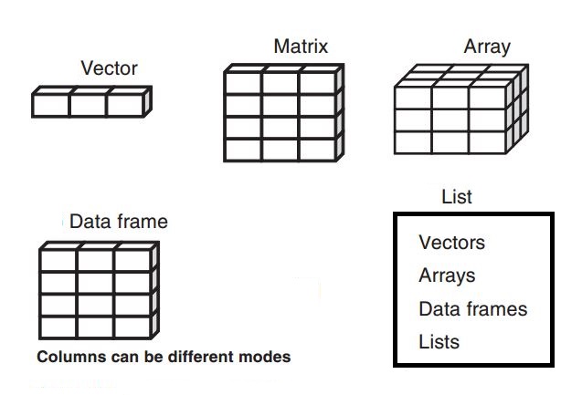
library(tidyverse)

1. Vectors

A vector is a one-dimensional, ordered collection of elements. A key characteristic of vectors is that all elements must be of the same data type (homogeneous). They are the simplest and most common data structure in R.

Creating Vectors

Vectors are typically created with the c() (combine) function.

Code

# A numeric vector
numeric_vector <- c(10.5, 2.3, 15.0, 4.8)
numeric_vector

[1] 10.5  2.3 15.0  4.8

Code

# A character vector
character_vector <- c("apple", "banana", "cherry")
character_vector

[1] "apple"  "banana" "cherry"

Code

# A logical vector
logical_vector <- c(TRUE, FALSE, TRUE, TRUE)
logical_vector

[1]  TRUE FALSE  TRUE  TRUE

Sequence Vector

The seq() function generates a sequence of numbers.

Code

seq(from = 2, to = 14, by = 2)

[1]  2  4  6  8 10 12 14

Replicated Vector

The rep() function repeats a value a specified number of times.

Code

rep(x = 1.5, times = 4)

[1] 1.5 1.5 1.5 1.5

Random Vector

The sample() function takes a random sample from a set of elements. replace = FALSE means each element can only be chosen once.

Code

sample(1:10, 5, replace = FALSE)

[1]  3  5 10  7  4

With replace = TRUE, elements can be chosen multiple times.

Code

sample(1:10, 5, replace = TRUE)

[1] 10  7  4  8  4

runif() generates random numbers from a uniform distribution.

Code

runif(1, min = 0, max = 1)

[1] 0.7881073

rnorm() generates random numbers from a normal distribution.

Code

sn1 <- rnorm(4, mean = 0, sd = 1) # Standard normal distribution
sn1

[1] -1.4745783 -1.9213412  0.7861794  1.6874680

Unique Vector

The unique() function removes duplicate elements from a vector.

Code

v1 = c(1, 1, 2, 2, 5, 6)
v1

[1] 1 1 2 2 5 6

Code

unique(v1)

[1] 1 2 5 6

Type Coercion

If you try to mix types, R will coerce the elements to the most flexible type in a specific hierarchy: logical -> integer -> numeric -> character. For example, mixing numbers and characters will result in a character vector because character is the most flexible type.

Code

mixed_vector <- c(1, "apple", 3.5, TRUE)
class(mixed_vector) # All elements are now characters

[1] "character"

Code

mixed_vector

[1] "1"     "apple" "3.5"   "TRUE"

Vector Operations

Mathematical and logical operations on vectors are performed element-wise. This is a powerful feature called vectorization, which is much faster than writing a loop.

Code

a <- c(1, 2, 3)
b <- c(10, 20, 30)

a + b # Element-wise addition

[1] 11 22 33

Code

a * 10 # Scalar multiplication is applied to each element

[1] 10 20 30

Subsetting Vectors

You can select elements from a vector using their index inside square brackets []. R uses 1-based indexing.

Code

character_vector[2] # Select the second element

[1] "banana"

Code

numeric_vector[c(1, 3)] # Select the first and third elements

[1] 10.5 15.0

Code

numeric_vector[numeric_vector > 10] # Select elements based on a logical condition

[1] 10.5 15.0

Code

# You can also exclude elements using negative indices
numeric_vector[-2] # Exclude the second element

[1] 10.5 15.0  4.8

Append Vector

You can combine vectors by using the c() function.

Code

x = c(1, 2, 3)
y = c(4, 5, 6)
z = c(x, y)
z

[1] 1 2 3 4 5 6

Remove Elements from a Vector

Negative indexing removes elements at the specified positions.

Code

x = c(1, 2, 3, 4, 5)
x

[1] 1 2 3 4 5

Remove the first element:

Code

x[-1]

[1] 2 3 4 5

Remove the last element:

Code

x[-length(x)]

[1] 1 2 3 4

Remove elements based on a vector of indices:

Code

remove = c(2, 4)
x[-remove]

[1] 1 3 5

Sort Vector

sort() arranges vector elements in ascending or descending order.

Code

a = c(2, 4, 6, 1, 4)
sort(a)

[1] 1 2 4 4 6

Code

sort(a, decreasing = TRUE)

[1] 6 4 4 2 1

Vector Length

length() returns the number of elements in a vector.

Code

length(a)

[1] 5

Vector Calculation

Mathematical functions can be applied to entire vectors.

Code

x = c(1, 2, 3, 4, 5)
sum(x)

[1] 15

Select Vector Elements

Code

x = c(1, 2, 3, 6, 9, 10)

Select the first element:

Code

x[1]

[1] 1

Select the last element:

Code

x[length(x)]

[1] 10

Select a range of elements:

Code

x[1:3]

[1] 1 2 3

Compare Two Vectors

setdiff(x, y) finds elements that are in vector x but not in vector y.

Code

xx = c(1, 2, 3, 4)
yy = c(2, 4)
setdiff(xx, yy)

[1] 1 3

Converting Between Vector Types

as.* functions are used to coerce vectors from one type to another.

Code

x <- c("a", "g", "b")
y = as.factor(x)
y

[1] a g b
Levels: a b g

Code

x <- c('123', '44', '222')
y = as.numeric(x)
y

[1] 123  44 222

2. Data Frames

A data frame is a two-dimensional, heterogeneous data structure, similar to a spreadsheet or a SQL table. It is the most important data structure for data analysis in R.

Each column is a vector.
Each column can have a different data type.
All columns must have the same length.

Creating Data Frames

Use the data.frame() function or, preferably, the tibble() function from the tidyverse. Tibbles are a modern take on data frames that are more user-friendly: they don’t change variable names or types, and they have a much nicer print method.

Code

my_df <- tibble(
  id = 1:4,
  name = c("Alice", "Bob", "Charlie", "David"),
  score = c(95, 82, 78, 91),
  is_student = c(TRUE, FALSE, TRUE, FALSE)
)

my_df

# A tibble: 4 × 4
     id name    score is_student
  <int> <chr>   <dbl> <lgl>     
1     1 Alice      95 TRUE      
2     2 Bob        82 FALSE     
3     3 Charlie    78 TRUE      
4     4 David      91 FALSE

Subsetting Data Frames

You can subset data frames in several ways:

$ or [[ ]] to select a single column by name. This returns the column as a vector.
[row, column] to select specific rows and columns. The result is another data frame (or a vector if you select a single column).

Code

# Select the 'name' column (returns a vector)
my_df$name

[1] "Alice"   "Bob"     "Charlie" "David"

Code

# Select the first two rows and the 'name' and 'score' columns (returns a tibble)
my_df[1:2, c("name", "score")]

# A tibble: 2 × 2
  name  score
  <chr> <dbl>
1 Alice    95
2 Bob      82

For more complex subsetting, it is highly recommended to use the dplyr verbs filter() and select() (covered in a separate guide).

Data Frame to Matrix

Converting a data frame to a matrix will coerce all elements to the most flexible data type (usually character).

Code

mat <- as.matrix(my_df)
mat

     id  name      score is_student
[1,] "1" "Alice"   "95"  "TRUE"    
[2,] "2" "Bob"     "82"  "FALSE"   
[3,] "3" "Charlie" "78"  "TRUE"    
[4,] "4" "David"   "91"  "FALSE"

Data Frame to Vector

You can extract a single column as a vector using $ or [[ ]] notation.

Code

vec = my_df[['name']]
vec

[1] "Alice"   "Bob"     "Charlie" "David"

3. Matrices

A matrix is a two-dimensional, homogeneous data structure. All elements must be of the same type. It is most useful for mathematical and statistical operations, such as linear algebra.

Creating Matrices

Use the matrix() function.

Code

my_matrix <- matrix(
    data = 1:12,      # The data to fill the matrix
    nrow = 3,         # The number of rows
    ncol = 4,         # The number of columns
    byrow = TRUE      # Fill the matrix row by row (default is by column)
)

my_matrix

     [,1] [,2] [,3] [,4]
[1,]    1    2    3    4
[2,]    5    6    7    8
[3,]    9   10   11   12

Subsetting Matrices

Subsetting is similar to data frames, using [row, column] notation.

Code

my_matrix[2, 3] # Element in the 2nd row, 3rd column

[1] 7

Code

my_matrix[1, ] # The entire 1st row

[1] 1 2 3 4

Code

my_matrix[, 4] # The entire 4th column

[1]  4  8 12

Matrix Operations

Matrices support matrix algebra operations, such as transposition (t()) and matrix multiplication (%*%).

Code

t(my_matrix) # Transpose the matrix

     [,1] [,2] [,3]
[1,]    1    5    9
[2,]    2    6   10
[3,]    3    7   11
[4,]    4    8   12

4. Lists

A list is a one-dimensional, heterogeneous data structure. Unlike vectors, lists can contain elements of different types and even different structures, including other lists, vectors, or data frames. This makes them very flexible, like a container for other objects.

Creating Lists

Use the list() function. It’s good practice to name the list elements.

Code

# A list is often used to return multiple results from a function
my_model_output <- list(
  name = "Linear Model",
  coefficients = c(intercept = 2.5, slope = 0.8),
  r_squared = 0.85,
  data = head(mtcars)
)

my_model_output

$name
[1] "Linear Model"

$coefficients
intercept     slope 
      2.5       0.8 

$r_squared
[1] 0.85

$data
                   mpg cyl disp  hp drat    wt  qsec vs am gear carb
Mazda RX4         21.0   6  160 110 3.90 2.620 16.46  0  1    4    4
Mazda RX4 Wag     21.0   6  160 110 3.90 2.875 17.02  0  1    4    4
Datsun 710        22.8   4  108  93 3.85 2.320 18.61  1  1    4    1
Hornet 4 Drive    21.4   6  258 110 3.08 3.215 19.44  1  0    3    1
Hornet Sportabout 18.7   8  360 175 3.15 3.440 17.02  0  0    3    2
Valiant           18.1   6  225 105 2.76 3.460 20.22  1  0    3    1

Subsetting Lists

Subsetting lists requires understanding the difference between [ and [[:

[[index]] or [[name]] extracts a single element from the list. The result will have the type of that element.
[index] or [name] extracts a sub-list. The result is always another list, even if you only select one element.

Code

# Extract the 'coefficients' vector (result is a numeric vector)
my_model_output[["coefficients"]]

intercept     slope 
      2.5       0.8

Code

# Extract a sub-list containing only the 'coefficients' element (result is a list)
my_model_output["coefficients"]

$coefficients
intercept     slope 
      2.5       0.8

Code

# Use the $ operator as a convenient shortcut for [[name]]
my_model_output$r_squared

[1] 0.85

5. Arrays

An array is a multi-dimensional, homogeneous data structure. It can have two or more dimensions. A 2D array is essentially a matrix. Arrays are useful for storing data that has more than two dimensions, such as image data (height, width, color channels) or time series data for multiple locations.

Creating Arrays

Use the array() function, specifying the data and the dimensions.

Code

# Create a 3D array (2 rows, 3 columns, 2 layers)
my_array <- array(
  data = 1:12, 
  dim = c(2, 3, 2)
)

my_array

, , 1

     [,1] [,2] [,3]
[1,]    1    3    5
[2,]    2    4    6

, , 2

     [,1] [,2] [,3]
[1,]    7    9   11
[2,]    8   10   12

Subsetting Arrays

Elements are accessed using [row, column, dimension] notation.

Code

# Element in the 1st row, 2nd column of the 2nd layer
my_array[1, 2, 2]

[1] 9

Code

# The entire first matrix (1st layer)
my_array[, , 1]

     [,1] [,2] [,3]
[1,]    1    3    5
[2,]    2    4    6

6. Inspecting Data Structures

Understanding the structure of your data is a critical first step in any analysis. R provides several useful functions for this.

str(): The most useful function. Provides a compact, human-readable summary of any R object.
class(): Returns the high-level class of an object.
typeof(): Returns the internal storage type.
length(): Returns the number of elements in a vector or list.
dim(): Returns the dimensions (e.g., rows and columns) of a data frame, matrix, or array.
names() or colnames(): Returns the names of elements or columns.

Code

str(my_df)

tibble [4 × 4] (S3: tbl_df/tbl/data.frame)
 $ id        : int [1:4] 1 2 3 4
 $ name      : chr [1:4] "Alice" "Bob" "Charlie" "David"
 $ score     : num [1:4] 95 82 78 91
 $ is_student: logi [1:4] TRUE FALSE TRUE FALSE

Code

str(my_model_output)

List of 4
 $ name        : chr "Linear Model"
 $ coefficients: Named num [1:2] 2.5 0.8
  ..- attr(*, "names")= chr [1:2] "intercept" "slope"
 $ r_squared   : num 0.85
 $ data        :'data.frame':   6 obs. of  11 variables:
  ..$ mpg : num [1:6] 21 21 22.8 21.4 18.7 18.1
  ..$ cyl : num [1:6] 6 6 4 6 8 6
  ..$ disp: num [1:6] 160 160 108 258 360 225
  ..$ hp  : num [1:6] 110 110 93 110 175 105
  ..$ drat: num [1:6] 3.9 3.9 3.85 3.08 3.15 2.76
  ..$ wt  : num [1:6] 2.62 2.88 2.32 3.21 3.44 ...
  ..$ qsec: num [1:6] 16.5 17 18.6 19.4 17 ...
  ..$ vs  : num [1:6] 0 0 1 1 0 1
  ..$ am  : num [1:6] 1 1 1 0 0 0
  ..$ gear: num [1:6] 4 4 4 3 3 3
  ..$ carb: num [1:6] 4 4 1 1 2 1

7. Choosing the Right Data Structure

Use a…	When you have…	Example Use Case
Vector	A 1D sequence of the same data type.	A single column of data, like ages or names.
Data Frame	A 2D table with columns of different data types.	Your typical dataset for analysis.
Matrix	A 2D grid of the same data type.	A correlation matrix, an image grayscale matrix.
List	A collection of different types/structures.	To return multiple, varied objects from a function.
Array	A multi-dimensional grid of the same data type.	3D medical imaging data, climate data over time.

1. Vectors

Creating Vectors

Sequence Vector

Replicated Vector

Random Vector

Unique Vector

Type Coercion

Vector Operations

Subsetting Vectors

Append Vector

Remove Elements from a Vector

Sort Vector

Vector Length

Vector Calculation

Select Vector Elements

Compare Two Vectors

Converting Between Vector Types

2. Data Frames

Creating Data Frames

Subsetting Data Frames

Data Frame to Matrix

Data Frame to Vector

3. Matrices

Creating Matrices

Subsetting Matrices

Matrix Operations

4. Lists

Creating Lists

Subsetting Lists

5. Arrays

Creating Arrays

Subsetting Arrays

6. Inspecting Data Structures

7. Choosing the Right Data Structure

8. Reference